| State | Seats | 110th congress average(Q) |
|---|---|---|
| MD | 8 | 150.3 |
| NC | 13 | 115.5 |
| FL | 25 | 90.4 |
| PA | 19 | 89.1 |
| CA | 53 | 80.6 |
| NJ | 13 | 77.6 |
| IL | 19 | 76.6 |
| TX | 32 | 68.6 |
| AL | 7 | 64.8 |
| TN | 9 | 62.9 |
| MA | 10 | 62.0 |
| VA | 11 | 55.7 |
| NY | 29 | 54.9 |
| OH | 18 | 51.0 |
| The 14 US states with average(Q)>50 during 2007-2008. | ||
By Brian Olson & Warren D. Smith. Third PRELIMINARY draft August 2011.
There is no issue that is more sensitive to politicians of all colors and ideological persuasions than redistricting. It will determine who wins and loses for eight years.
– Ted Harrington, chair of political science at the University of North Carolina (quoted during Shaw v. Hunt trial, March 1994).
Smith was urged to write an essay about theoretical issues in political districting. This page is his current answer to this request. Brian Olson helped him a lot hence is credited as co-author.
At any level of government, a district means that there is a specific piece of government responsible for your and the other people in your district's needs. Districts break governance into managable pieces. School districts let us manage just the schools 'here' and not 'there.' State Legislature and Congressional districts let you elect one specific representative.
"Democracy" is voters choosing their leaders. But when politicians get to draw their own districts, such as (most egregiously) in the USA, the result is the opposite – the politicians choose their voters. Outrageously biased absurd-looking district maps are common in the 2000-era USA, and not coincidentally, re-election rates to congress are ≈98%. Voters thus play little role in the "democratic" process. Statehouses often are even worse.
Here's an actual quote (given as evidence in a court case) by a redistricting committee chairman to one of his committee colleagues: "We are going to shove [this map] up your f------ a-- and you are going to like it, and I'll f--- any Republican I can."
US Supreme Court Justice Sandra Day O'Connor apparently regarded this as a virtue, opining that any politician who did not do absolutely everything he could to help his party "ought to be impeached." (To be clear, the fact that a US supreme court justice could emit that quote, absolutely astounds and revolts me; and I would be more in agreement with "any politician who does absolutely everything he can to help his party ought to be impeached.")
Justin Levitt (Law Professor at Loyola) claims that the USA "is unique among industrialized democracies in putting an inherent conflict of interest directly at the heart of the redistricting system."
Computerized gerrymandering systems and massive secret databases about people compiled by the political parties (they know your gender, your household composition, what magazines you subscribe to, what party you are registered in, what crimes you committed, how often you vote, what products you buy...) are now enabling gerrymandering with extreme levels of detail – individual buildings – making the problem much worse still. This all is an extreme failure of democracy.
Stupid ways to try to avoid this problem, which in the USA usually have not worked, include
I know of exactly two ways to genuinely fix the problem and produce genuinely unbiased district maps.
Anybody in the world is allowed to run the same algorithm on the same data (both being public) to hopefully get the same district map, verifying there was no cheating, and if it is a simple-enough algorithm then anybody can check validity to a considerable extent just "by eye" with no computer needed. In the results-based paradigm, again, anybody can confirm the claimed map goodness by computer, or, if it is a simple-enough quality definition, one can confirm/deny fairly well merely by eye.
Why can't we get the best of both worlds by making a computer find the best possible district-map? Because for all three of my favorite reasonable quality metrics, I can prove that finding the best district-map [or even answering the yes/no question "does a map with quality better than X exist?"] is an "NP-complete" problem. (Discussed in NP-completeness section below.) Given that essentially everybody believes P≠NP, that basically means that there cannot be any computer program that both (i) finds the best map, or even merely answers that yes/no question for arbitrary X and (ii) can be guaranteed to run quickly enough that it is going to finish computing in any reasonable amount of time (e.g. your lifetime, the age of the universe, etc).
Note the word "guarantee." Even if some computer program were found by empirical testing to often succeed quickly in finding a provably optimum districting, there would be no guarantee that the very next run tried would not take longer than the age of the universe. This is unfortunately simply the way it is with NP-complete problems, and is why NP-completeness renders many schemes unacceptable for many election-related and districting-related purposes in which guarantees are required.
OK, can we at least make a computer find a map guaranteed to be no worse than a factor of 2 away from optimum? (Or a factor 1.1? Or 1.01? Or any constant factor at all, even 9999999?) Those at present (year 2011) all remain open questions for any of the three quality-measures discussed below! I suspect such an algorithm will eventually be found (indeed, I have some candidates), but unfortunately I also suspect it will be complicated.
Will that contest paradigm work in real life? I'm presently unconvinced. There was a trial contest to redistrict Arizona 2011, and it was a total failure; by their announced deadline 5 June nobody was able to use their website's software to produce any sensible map (there were a few "entrants" which were obviously just failed experiments in using their software) whereupon they magically changed the deadline to 22 June. There was a later magical rescheduling too. I personally tried to use their contest software and failed, and so did several others whom I know. There would need to be hundreds, maybe thousands or tens of thousands, of such contests set up to district all the 100s-10000s of areas that need to be districted. MORE ON THIS???
The whole paradigm depends on having enough entrants (and enough entrants with enough competence!) in every contest. Right now, often, even simple manual sanity checks on published-by-the-USA-government election results, simply are not conducted. Not by any person. Not by any group. Not even the losing candidates in that election, even in close races, perform simple arithmetic sanity checks!! I know this because, many years later, when I or somebody else gets prodded by some random news event to finally perform such a sanity check, we often find some incredibly obvious mathematical impossibility (often more than one). Like more votes than voters. Or sums that are wrong. With these errors exceeding the official election margin. Meaning nobody ever found it/them and made it/them public before. CITE EXAMPLES??? Now drawing district maps is far more complicated and difficult than performing simple arithmetic checks on published election results. It's pretty much beyond the ability of some unfunded amateur without computerized tools. So it is even less likely to happen.
But in the future, computerized tools will get common and huge numbers of people will enter the contests, right? Maybe they will and maybe they won't. Even if you can easily get and install such tools and they all work perfectly and you aren't worried their authors might be evilly trying to malware your computer – it still is way easier to perform simple sanity checks on election results, and I repeat, that isn't happening. And the government can and often has in the past, published their data in bizarre, changing with time and place, formats. (With errors in it too.) For example just now for 2010 the census department changed its file formats, killing our districting program (which had worked with their 2000-era data). Election data all over the USA is published in absolutely insane, ridiculous, not the same in this town as that town, formats, making it impossible for any simple computer tool to just look at everything on election day and spot obvious insanities. It can take hours to months to rewrite your program to try to eat some new data format, and months of effort per town, with tens of thousands of towns in the USA, adds up to too much effort. In short, the politicians could easily screw up any contest to make it effectively impossible for anybody to enter it besides their own entrant. Just like they made "Jim Crow" laws which for 50+ years made it almost impossible for black people in the Southern USA to vote. Just like they have blatantly gerrymandered, drawing absolutely absurd district-shapes, for 200+ years without ever stopping, now having ≈98% re-election rates. Just like the Tweed Ring took over New York and redirected about one-third of its total budget into their own pockets, with only 2 members of this ring ever serving any jail time ever.
But we'll just solve that problem by making a law that there has to be a simple, never-changing, fixed format for census and map data. Dream on. Let me put it this way. In the history of the universe, I doubt there has ever been such a law, and trying to describe data formats in legalese basically adds up to dysfunctional garbage.
As of 2011, there is an ISO standard for "Geographic information – Geodetic codes and parameters" (ISO/TS 19127:2005) but unfortunately there do not appear to be any ISO standards for "census" or "population" or reporting election results.
Incidentally, we wrote a program to eat 2000 USA census data... and the census dept swore to us they'd never change this data format. It was a de facto standard which tons of software all over the world relied on. So they'd never change it. Presto, very next census (2010) they changed it and all the old software broke.
Will the procedure-based paradigm work in real life? Yes it will. The government itself will need to run the procedure so they will not be able to stop contestants by introducing bogus and sick data, because they are the only contestant. Even if the government decides to stall and claim it was impossible for them to produce a district map, then other people could easily run the algorithm so everybody would know what the map was anyway. Gerrymandering will be impossible because the algorithm produces one and only one map, with no adjustability whatsoever, given your state's shape and where its people live. Ivan Ryan programmed the shortest splitline algorithm and ran it on all 50 US states using year-2000 US census data – at a cost in electricity of around 10 cents and total computer runtime (needed only one 2000-era PC) of one day, which are far less cost and time than the USA's human districters have ever consumed – and it almost always produced clearly-better district maps.
Here are three quality-measures that previous authors have proposed as hopefully suitable for the contest-based paradigm or evaluative purposes. (In all cases, we demand there be exactly N districts, all equi-populous, and each a connected set.)
About "equipopulousness": It is mathematically feasible, but in the real world infeasible and pointless due to census data-gathering errors, to get exact equi-populousness down to at most ±1 person. Requiring the max-pop district have ≤1.005 times the alleged population of the min-pop district plus at most 5 people, seems a more-than-adequate compromise sanctioned by US courts, although 0.7% deviation was judged too much in KARCHER vs. DAGGETT 1983.1. Brian Olson's "average distance to center" measure:
Across all districts and all people, the "best" district map is the one where people have the least average distance to the center of their district. (And this quantity – the average distance from a person to her district-centerpoint – is a numerical measure of goodness for any map; smaller numbers are better.) Note, a similar but much worse idea was put forward by Boyce & Clark 1964.
Annoying but crucial details: "Distance" means geodesic "great circle" distance on the surface of the sphere. This distance between two points with (longitude, latitude) given by (a,b) and (c,d) is
where R≈6371km is the radius of the Earth and |b-d| is computed appropriately modulo 360 so that it always is ≤180 degrees. "Center" means, I presume, the "Fermat-Steiner-Weber point" (based on surface-distance) of all the people-locations in that district. The FSW point of N point-sites is defined to be the point X which minimizes the sum of the N distances from X to the sites. There are known efficient algorithms to find X to high accuracy (it's a "convex programming" problem), although these algorithms are not obvious and not very simple. On a flat earth the FSW point is always unique. On a round earth it can be non-unique, but that should not be a problem in practice.
To learn more about FSW points:
http://en.wikipedia.org/wiki/Geometric_median
http://en.wikipedia.org/wiki/Fermat_point
http://mathworld.wolfram.com/FermatPoints.html.
"Weiszfeld's iteration" consists of iteratively replacing the current center X (initially a random point) by the weighted mean of all the sites, where the weight of site k is proportional to the reciprocal of its distance to the current X. (The proportionality constant is chosen so the weights sum to 1.) In a Euclidean space using ordinary Euclidean distance, X converges to the FSW point – in a manner which decreases the summed distance each iteration – provided the sites have a full-dimensional convex hull and provided X never lands exactly on a site. (References on Weiszfeld iteration.)But on a round Earth using surface distance, it's a little more difficult. The following new Weiszfeld-like algorithm conjecturally works if all the sites lie within the same hemisphere: work in a suitable gnomonic projection of the Earth's surface onto a flat plane. (The virtue of this map projection for districting purposes is that geodesic shortest-paths on the sphere correspond to straight line segments on the plane, hence "convexity" is preserved.) On this flat map, use the Weiszfeld iteration, but letting the weight of site k instead be proportional to
EuclideanDist(X, sitek)-2TrueSphericalDist(X, sitek). Finally, after X has converged, un-project it back onto the sphere.
Side-note on the gnomonic projection: To map (x,y,z) on the unit sphere (x²+y²+z²=1) to (X,Y) in the plane via a gnomonic projection centered at a point C having longitude=A and latitude=B, first rotate (x,y,z) about the North-South z-axis by angle -A so that C is moved onto the Greenwich meridian at x=1; then rotate by angle -B about the y-axis to move C onto the equator with z=0 [the net effect is to move C to new location (1,0,0)]:[ x ] [ cosB 0 sinB ] [ cosA sinA 0 ] [ x ] [ y ] ← [ 0 1 0 ] [ -sinA cosA 0 ] [ y ] [ z ] [ -sinB 0 cosB ] [ 0 0 1 ] [ z ] new rotation by rotation by old xyz angle -B angle -A xyz[now it should be the case that x>0 otherwise (x,y,z) was on the other side of the planet from C] then perform the projection itself:X = y/x; Y = z/x. This last operation can be inverted by x=(1+X2+Y2)-1/2 then y=xX, z=xY.I note that the direction to the Weiszfeld point is always a descent direction (also true for Cooper 1968's variant based on distancee rather than plain distance, for any exponent e with 1≤e<∞; and also true for our gnomonic-projected version of the spherical-distances problem; this using Cooper's or my generalized Weiszfeld iterations) so that one can always "back up" from the candidate new Weiszfeld point by repeatedly dividing the stepsize by 2 until we find a descent point.
Relation to Average Interperson Distance: The average distance from a random person to a random person in the same district, is bounded between 1 and 2 times Olson's average distance to district-center.
Olson's motivation: If there were exactly one voting-place in each district, and if each one were optimally located, and if each inhabitant traveled there by personal helicopter to vote, and if all helicopters had identical performance, then the best district map by Olson's criterion, would be the one minimizing the total travel expense to all the people each election. But of course in real life all these "if" assumptions are untrue, especially the first. They may, however, have some approximate validity.
2. The "average squared-distance" (area-valued) measure:
The "best" district map is the one where the average squared-distance between two people in the same district (averaged across all districts and all such people-pairs) is minimized.
I intend that "squared distance" now mean
the usual Pythagorean straight-line formula.
To convert from (longitude,latitude) pair (α,β) to Euclidean coordinates (x,y,z) use x=[cosα][cosβ], y=[sinα][cosβ], and z=sinβ.Remarks: It is mathematically equivalent (but simpler to compute) to minimize the average squared-distance between each person and her district-centerpoint, where "center" now simply means the numerical average (in 3-space) of all the (x,y,z) locations of the voters in that district. (It is well known that the average of sites in a Euclidean space uniquely minimizes the sum of squared distances to those sites.) This quantity is a numerical quality-measure for any districting (smaller numbers better). It has the dimensions of squared distance, i.e. area, as opposed to Olson's measure which has the dimensions of length.
The reasons it is "simpler to compute" this than Olson's measure are
- because squared Euclidean distances are simpler to compute than unsquared surface distances (no trig, inverse-trig, or square roots required; just multiply, add, & subtract)
- averages are much simpler to compute than FSW points.
Olson should easily be able to modify his computer program to employ either quality measure 1 or 2 (user chooses which).
The reason the pair-sum and single-sum measures are "equivalent" is that
∑1≤i≤N ∑1≤j≤N (xi-xj)2 and 2N ∑1≤i≤N (xi-μ)2 where Nμ = ∑0≤j≤N xj are identical and N (the population of a district) is merely a constant scaling factor. To prove that, realize that both expressions are translation-invariant, i.e. adding any fixed constant vector to all the xi and to μ leaves both of our expressions unaltered, so therefore we can wlog demand μ=0=∑jxj, whereupon it becomes trivial to see they're equal.
3. The min-perimeter measure:
The "best" district map minimizes the total length of all the district boundaries (subject to the usual constraints that there be the correct total number of districts and each have the right population and form a connected set). This total length is a quality measure for any map (smaller is better).
This tends to prevent ultra-wiggly district boundaries and makes maps easy to draw. It is probably the easiest measure (among the three) to compute. It also tends (albeit somewhat less directly) to minimize voter travel distances.
Mackenzie's related index: John Mackenzie in his paper Gerrymandering and Legislator Efficiency introduced the following measure Q of badness, which some have branded the "Mackenzie index":
Let P=g+n denote total district perimeter as the sum of mutable political boundary length g plus immutable natural boundary length n. The the mutable proportion equals g/P. The polygon complexity attributable to political manipulation is Q = (g/P)(P2/A) = gP/A.
For districts with g=P, the least possible Mackenzie index would be achieved on a flat earth by a circle, with Q=4π≈12.57; a square would have Q=16; a 2×1 rectangle would have Q=18; a 3-4-5 right triangle would have Q=24; and a 4×1 rectangle would have Q=25. Therefore in my opinion districts with Q>40 ought to be illegal. But Q values as low as 0 are possible (for a state consisting of exactly 1 district, entire boundary immutable) and unboundedly large values also are possible (very wiggly boundary). The worst districts in the 1999-2009 USA had 200<Q<900.
Mackenzie then used US government district shape datafiles to compute all Q values for all congressional districts for the 106th through 110th congresses (years 1999-2008) and used the results to create color coded maps of the USA highlighting the worst-gerrymandered areas (100<Q≤870) in orange and red, and the least-gerrymandered areas (0≤Q≤75) in green. The worst-gerrymandered states during this era (having greatest average Q for their districts), are given in the table below at left computed by Mackenzie (2007-2008 only); at right are Mackenzie's five Q-maps combined into one animated GIF, and note that about half the land area of the USA is gerrymandered at Q>50 levels which I contend ought to be illegal.
|
| ||||||||||||||||||||||||||||||||||||||||||||||||
Gerrymandertude changes with time. In the earlier 106th congress (1999-2000) it looks to the eye like the most-gerrymandered states instead were
in approximately worst→best order.
Mackenzie then also tried to ask: "Is there any correlation (or anti-correlation) between the geometric complexity (Q value) of districts and the efficacy of their congressmen at unfairly channeling federal money toward that district?" But he failed to find any such connection (or if one exists, then it is not immediately apparent in his data, the "noise" seeming larger than the "signal").
Generically unique optimum Theorem: each of the above three measures generically yields a unique optimum partitioning of the P people into N districts for any P≥N≥1 (max-pop district has at most 1 more person than min-pop district; "people" regarded as disjoint points on the sphere surface). "Generic" means if the people's locations got perturbed randomly-uniformly by ≤ε then you'd get uniqueness with probability=1 for any ε>0, no matter how small, starting from any set of people locations.
Proof:
Assume a flat Earth.
"Generic real numbers" disobey every polynomial equation with integer coefficients
(except for always-true equations such as 1=1). In other words they
are "algebraically unrelated."
For any partitioning of the P points
into N equi-populous subsets we can compute the centerpoints (whether mean or FSW-point)
for each subset and thus its Olson or squared-distance-based quality measure, as an
algebraic
function of the people's coordinates. Since no two algebraic functions can be equal
on generic data (because if they were, you'd get one of those forbiddden polynomial equalities),
these quality measures will have distrinct values for
every partitioning, and hence the optimum partition must generically be unique.
The perimeters-sum measure also is an algebraic function of the coordinates
(for any given partition), and a different function for each partition; so
no two partitions can have equal cost, so again the optimum is
generically unique.
For a round Earth, one can employ e.g. the stereographic projection to "flatten" it,
but then the above proof only immediately works for the sum-of-squared-based measure, because only
it is an algebraic function of the flat-map coordinates (the other two measures
also require inverse-trigonometric functions). It is, however, possible by using trigonometric
"summed angle" identities to convert any cost-equality
into an algebraic (and then further into a polynomial)
equality. For example if two sums of arccosines are equal, then take the cosine of both sides,
and apply cos(A+B)=cos(A)cos(B)-sin(A)sin(B) and use
sin(A)2+cos(A)2=1 and cos(arccos(X))=X to convert to an algebraic identity.
Q.E.D.
Another way to prove all this is to note that the number of possible ways to write
cost-equality formulae
is at most countably infinite, whereas the real numbers are uncountably infinite;
it is key that for our cost-measures any two set-partitions always have different
cost-formulae.
Of course with special (non-generic) real numbers, it is possible for two different districtings to be exactly tied for least-cost. The virtue is that any slight perturbation of the people-locations will (with probability 1 for a random perturbation) break all ties.
The following inequalities hold where "optimal" means the least-cost map for that cost measure, i.e. each occurrence of the word "optimal" has a different meaning:
Note the middle inequality is only valid if "distances" are measured in the same way on both sides of it (but sadly Spherical & Euclidean distances differ) but the outer two "≤"s are valid even using the two different kinds of distances involved in our quality definitions. The middle ≤ becomes valid with our incompatible distances either in the flat-Earth limit or if we weaken it by multiplying its left hand side by (2/π).
Proof: The distance from A to B cannot exceed half the perimeter of the district (A,B both in the district) as you can see by rigidly moving AB until both endpoints hit a boundary. Hence the square root of the mean squared distance to center, is ≤ the square root of the maximum squared distance to center, which is ≤ perim/2. Of course, that is for the districts that minimize perimeter. For the districts redrawn to minimize mean-squared-distance, this inequality only becomes more true; and if we switch from spherical surface distance to Euclidean 3D distance, it again only makes it more true since the latter kind of distance is always smaller. Next, for any set of nonnegative real numbers, their mean is always ≤ the square root of their mean square. Of course, that is for the districts that minimize mean-squared-distance. Redrawing the districts to minimize mean-unsquared-distance, only makes the inequality more true. If the squared distances are measured using straight line 3D distance but the unsquared distances are measured on the sphere surface, then that reasoning was invalid but is salvaged if we weaken it by multiplying the left hand side by (2/π) because straight-line 3D distances from A to B cannot be shorter than (2/π) times the sphere surface distance from A to B (and equality occurs only if A and B are antipodal). Q.E.D.
It is possible by positioning the people appropriately to make each of these ≤ be very strongly obeyed, i.e. "<<"; but with a uniform distribution of people in any nicely-shaped country, the three quantities all will be within constant multiplicative factors of any other.
The above three quality-measures seem to me to be the best three among those that people have proposed over the years (that I am aware of). However, many stupid quality-measures have also been proposed. Many of them are incredibly stupid to the point where my mind absolutely boggles that professional scientists could actually have proposed them in print.
Example stupid idea #1: The "quality" of a district is the ratio of the radius of the smallest-enclosing circle, divided by the radius of the largest-enclosed circle (smaller ratios better).
Example stupid idea #2:
The "quality" of a district is the ratio of the area of the
smallest-enclosing circle, divided by the area of the district
(smaller ratios better). This has been called the "Roeck (1961) measure."
An even more-peculiar related quality measure was
Schwartzberg 1966's – defined on p.108 of
Young's review
paper as
the ratio of
a polygonal pseudo-perimeter divided by
the perimeter of a circle with the same area as the district.
This, because it is based on a polyonal pseudo-perimeter, is not affected
by the real perimeter. Thus in a district-map that is square grid with
500-mile sidelengths (not bad), replacing all the square sides by
arbitrary hugely-wiggly curves
would leave the Schwartzberg quality measure unaffected,
because (as defined by Young) the pseudo-perimeter would still be the original square grid!
I saw, however, a website which (re)defined Schwartzberg using genuine, not pseudo,
perimeter. Call that "sanitized Schwartzberg"; it makes far more sense.
(I do not have access to Schwartzberg's original 1966 paper.)
Example stupid idea #3: Inscribe the region in a rectangle with largest length/width ratio. This ratio is ≥1, with numbers closer to 1 corresponding to "better" regions. (Harris 1964 and Papayanopoulos 1973.)
In all cases the quality of the whole multi-district map is obtained by summing the qualities of all the districts within it.
A big reason these three ideas – and many others – are stupid, is that you can take a multi-district map "optimal" by this measure, then add a ton of essentially arbitrary wiggles to large portions of the district boundaries, while leaving the "quality" of that map exactly the same. Here's an example for stupid measure #1:
The picture shows a disc-shaped "country" subdivided by a diameter-line into two semicircular districts, one in the North and one in the South. This 2-district map is "optimum" by stupid quality measure #1 (dashed smaller circle is just a mental crutch to help you see that; it is not a district boundary; for how to know this is optimum, see Graham et al 1998 and employ the max≥arithmetic mean≥harmonic mean≥min inequality). However, upon making very-wiggly alterations to two portions of the interdistrict boundary as shown, we still have an "exactly optimum" 2-district map (assuming the original map was optimum) according to stupid measure #1. Similarly the hexagonal beehive ought to be optimum for both stupid quality measures #1 and #2, but we can alter large portions of each hexagon edge by adding almost arbitrary wiggles and still get an "exactly optimum" tesselation. Stupid idea #3 just does not work sensibly on a round Earth (there is no such thing as a "rectangle" if that means all four angles are 90 degrees; if it means all 4 angles are equal and the sides come in two equal-length pairs, then a district consisting of the entire Northern Hemisphere is "infinitely bad"!). If we only consider it on a flat Earth, then any region bounded by a constant-width curve (there are an continuum-infinite number of inequivalent such shapes) has ratio=1 and hence is "optimal" by stupid measure #3.
Example stupid idea #4: Yamada 2009 had the idea that the cost of a districting should be the total length of its minimum spanning forest; that is, for each district you find the minimum-length tree (MST) made of inter-person line segments for all the people in that district, and the cost of the whole districting is the sum of the lengths of all the district MSTs.
With Yamada's idea, if the people are located one each at the vertices of the regular-hexagon "beehive," then every district map (so long as each district contains a connected sub-network of the beehive) is "exactly optimum." This allows incredibly "fuzzy hairy tree shaped" districts while still achieving "exact optimality." There is virtually no discrimination. And presumably by perturbing these locations arbitrarily slightly we could break the tie in a highly arbitrary manner in which case insane fern-shaped districts would actually be "the unique optimum"!
Summary of stupidity: In other words, with those stupid quality measures
It's an embarrassing sign of the dysfunctionality of this entire scientific field, that, e.g. no previous author (before this web page) has considered the fundamental uniqueness theorems. In short, they never reached "square one."
It seems to me, however, that my three favorite quality measures are invulnerable to those criticisms – the "optimum" map is always a pretty decent map; and since it is generically unique any attempt to add wiggling to any boundary, will destroy optimality.
Example stupid idea #5: Quality of a district is the ratio of the area of the convex hull of a district divided by the area of the district.
Example stupid idea #6: Quality of a district is the probability that a district will contain the shortest path between a randomly selected pair of points in it. (Chambers & Miller 2007.)
Example stupid idea #7: An even stupider related idea – the average percentage of reflex angles in a polygonal pseudo-perimeter – was advanced by Taylor 1973.
With stupid ideas 5, 6 & 7, every convex shape is "exactly optimum." Thus the "hexagonal beehive" pictured in an upcoming section is optimum, but with this stupid idea so is the "squished beehive" with long thin needle-like districts (this picture was got by factor-2 squishing, but stupid ideas #5-7 would still regard this as "exactly optimum" even with 99!):
But Taylor's idea #7 goes beyond even that amount of stupidity to enter whole new regimes. Observe that Taylor's idea is not even defined for a district that is not polygonal (e.g. has boundaries that are smooth curves, or fractals). One could try to define it by approximating such a shape by a polygon, but then different sequences of polygons (all sequences approaching the same limit-shape) would yield vastly different Taylor quality measures. Thus, the Taylor measure is not a measure of shape at all!
Not necessarily. Some of them could still have value if used in combination with a non-stupid idea such as our three cost-recommendations. For example, we could minimize the sum of district perimeters (good idea #3) subject to the constraint that we only permit districts having ratio of the radius of the smallest-enclosing circle, divided by the radius of the largest-enclosed circle, less than 2 (stupid idea #1!) and/or subject to the constraint that we only allow convex district shapes (related to stupid ideas #5 and 6). (We then would need to use total district perimeters; i.e. we do not allow using segments of the country-border "for free"; indeed we in this formulation would need to ignore the country-border entirely, regarding the people-locations as the only important thing.)
I don't see anything wrong with this sort of idea-combination (aside from the fact that no district map satisfying the extra constraint exists, for, e.g, a very long thin country...), and indeed some such hybrid might be superior to either ingredient alone.
...the optimum way to subdivide it into equi-populous districts, would be a regular-hexagon "beehive" tessellation. (This is simultaneously true for all three of our optimality notions. For example using Olson's measure, the hexagon tesselation has average distance to tile-center which is approximately 98.5883% of what it would have been using the square-grid tessellation.)

However, on a round earth, or in a finite country, or with non-uniform population density, the pictures would change and would no longer (in general) be identical and no longer be the regular-hexagon-beehive.
The picture shows a disc-shaped "country," mainly rural, but with one densely-populated city (the small white off-center subdisc). The population densities in the city and rural areas both are uniform and both areas have equal total populations. For simplicity we use a flat Earth. The problem is to divide this country into exactly two districts.
Based on the above simple example – and also based on my intuition before I worked this example out – I suspect we have listed our three quality-measures in increasing order of both goodness and simplicity – the best one is the min-perimeter measure (3).
I'm not alone. Election-expert Kathy Dopp has also told me (June 2011) she independently came to the same conclusion for her own reasons: minimizing total perimeter is the best. More precisely (Oct 2011), it seems Dopp prefers to minimize some function of the isoperimetric ratios of the districts in the map. However, it is not clear to me what the best such function should be. See discussion below about "weighted sum." Similar ideas have been advanced also in many scientific publications by other authors.
Reasons:
In the contest paradigm, if you (a good person) submit a sensible districting, but I (evil) have more funding, hence more compute power and better programmers, than you, then I'll find a "better" map by either measure 1 or 2 (whichever is the one we are using). I will then be able to modify my map by adding an enormous number of evil wiggles, while still having a "better" map than you do (because that'll only alter my quality measure by a tiny amount which goes to zero like the square of the maximum wiggle-size when my wiggles are made small), hence I'll still win the contest.
To hammer that home: suppose I'm able to beat you by 1% due to my extra compute power. I'll keep my 1%-better map secret until 1 second before the contest deadline. I'll then add evil wiggles of order 10% of my district size to my map, and submit that. Note, I'll still be able to beat you, since the square of 10% is 1%. But wiggles of size 10% are actually quite enormous and quite sufficient to enable very severe gerrymandering! Evil will be able to win.
In practice the Democratic and Republican parties probably would have far more funding, compute-power, motivation, and programmer-years to throw at it than everybody else. Hence I worry that we might get an evil-Democrat plan or an evil-Republican plan always winning the contests, with the non-evil non-biased non-wiggly maps, all losing.
If we both are handed maps with N equi-populous districts, then I'll be able to evaluate the perimeter length without needing to know or think about the locations of every single person. All I need is a tape-measure. Meanwhile you, in order to compute quality-measures 1 and 2, will need to know, and do some arithmetic related to, the location of each of the millions of people. (Although actually I would need to know the people-locations if I wanted to be sure the districts were equi-populous; but not if all I wanted was to compute the cost-measure.)
However, I'm not 100% sure of the conclusion that min-perimeter is the best criterion.
This question of what is the best quality measure probably cannot be answered just via pure mathematics; it requires experiment. If somebody produced the optimum maps (for all three notions of "optimal") for districting about 100 real-world countries, and we looked at them, then we'd have a better idea how well they perform. As of the year 2011 nobody has done that experiment – and it would probably be infeasible to really do it since optimal districting is NP-hard – but see the pretty pictures section for the closest we've come.
But there are some valid counter-arguments that the min-squared-distance-based quality measure (2) is better than my favored min-perimeter measure (3). [And the new generalization of the concept of "Laguerre-Voronoi diagram" to nonEuclidean geometries can only bolster this view.] The case is not entirely one-sided:
A. Under certain rules (discussed below) the min-perimeter measure plausibly seems more vulnerable to manipulation by a (possibly corrupt) census department.
B. The squared-distance cost measure can easily be modified so that districts not only tend to be geographically compact, but also tend to group people with common interests together. To do that, associate an "interest vector" with each person. Each person now has more than 3 coordinates; the extra dimensions represent her interests. We now can use the same squared-distance-based cost measure as before, just in a higher-dimensional space. (I happen to hate that idea because: what qualifies as an "interest" and by how much should we scale each interest? Whoever arbitrarily decides those things, will control the world.)
C. The squared-distance-based measure has this beautiful property which in general is disobeyed by the other two:
Voronoi Characterization Theorem: The "optimum" N-district map according to the squared-distance-based measure always subdivides the population in such a way that the districts are "Voronoi regions." That is, associated with each district k, is a magic point xk in 4-space, such that the inhabitants of district k consist exactly of the people closer to xk than to any xj with j≠k. [Yes, I did say four-dimensional space! Use coordinates w,x,y,z. Every point on the Earth has w=0, but those N magic points are allowed to have w≥0. The x,y,z coordinates of a district's magic point are just the mean x,y,z for its inhabitants.]
Remark: This makes describing the exact shapes of the districts very simple – they always are convex polyhedra in 3-space – makes it easy for anybody to determine which district they are in (simply compute your N distances to the N magic points; which is closest tells you your district) – and finally makes it much easier for a computer to try to search for the optimum districting. Note also that if our districts are small enough that it is OK to approximate the Earth as "flat," i.e. 2-dimensional, then the regions are Voronoi regions whose magic points now lie merely in 3-space, and the Voronoi polyhedra, when we only look on the plane, reduce to convex polygons. In other words, on a flat Earth, the optimum N-district map always has convex polygonal districts. That's very nice.
Unfortunately on a round earth, it is not quite so simple. The optimum map's districts, although still convex polyhedra in 3-space, if just viewed on the sphere surface become usually-nonconvex "polygons" whose "edges" are non-geodesic circular arcs; and it is possible for a district to consist of more than one disconnected such polygons. For example consider N-1 equipopulous cities equi-spaced along the equator, plus two half-population cities at the North and South poles, plus a uniform distribution of a comparatively tiny number of rural people. The best N-district map (if N is sufficiently large) then has N-1 identical districts each containing a single equatorial city, plus an Nth district consisting of two disconnected regions containing both poles (all districts have equal area and equal population).
Even so, though, a very concise exact description of the optimum map exists – simply give the 4N coordinates specifying the N magic points. If we only permit thus-specified maps as contest-entrants, that prevents ultra-wiggly district boundaries, whereupon the criticism A of the sum-of-squares-based quality measure – that an evil computationally-powerful contest-entrant could submit a wiggly map and still win – is avoided.
Proof: See §5.3 of Spann, Gulotta & Kane for a beautiful proof employing the duality theorem for linear programming (which in turn is discussed in Dantzig 1963). Their -Cj is the same (up to an arbitrary overall additive constant) as our +wj2, and their pi is the "magic point" associated with district i, whose (x,y,z) coordinates, note, are seen to be the means of the people-locations in district i. Q.E.D.
Extension to handle Olson: The same Spann proof also will show a related theorem about what the Olson-optimum districting is: It always is an "additively weighted Voronoi diagram" for the sphere surface metric (basically you just go through their proof but now using unsquared distances). In other words, associated with each optimum-Olson district k is both a magic point Mk on the sphere surface (the FSW point) and a real "additive weight" Ak; and the kth optimal-Olson district consists precisely of the points x on the sphere such that
The regions in such a diagram are in general nonconvex (but always connected) and have boundaries described piecewise by certain algebraic curves. On a flat earth the district boundary curves are (piecewise) hyperbola-arcs and line segments; and the regions always are connected, although usually nonconvex.
(This section added 2018 by WDS.)
The above "Voronoi characterization theorem" describing the optimum districting (for quality measure 2 arising from sum-of-squared-Euclidean-distances from people to their district centerpoint) as a Voronoi diagram in a four dimensional space had several disadvantages on a round Earth. It turns out to be possible to eliminate those disadvantages by modifying the squaring function x→x2 slightly, as follows. We shall see exactly one (up to rescaling and additive offsets) "magic function" works.
Asterisk: in the spherical case, this theorem & corollary need only hold for Laguerre regions entirely containable within a single hemisphere. Indeed the whole Sugihara diagram concept breaks down if too-large districts, specifically those not containable within any single hemisphere, are permitted. Fortunately, I have checked that every continent, as well as the multicontinent Africa-Europe-Asia and N+S America contiguous land masses, each are containable within a single hemisphere. Therefore, on our planet this asterisk should not be much of a limitation.
The time has come to actually explain what this concept is.
The Sugihara/Smith nonEuclidean generalization of "Laguerre-Voronoi diagram." For N weighted point sites in a nonEuclidean space – each site k having a real-number-valued "weight" Wk – the diagram is the partition of the space into the N "Laguerre regions." Region k consists of all the points P of the space such that
for all j≠k. We have stated this magic formula using the magic function ln(sec(θ)) for the spherical-geometry case, where the NonEuclideanDistance is angular surface distance (i.e. "distance" from A to B is the angle subtended by A and B at the Earth's center). Note that sec(θ) is well behaved when 0≤θ<π/2, but sec(π/2) goes infinite. That is the reason for the "asterisk." If you instead want hyperbolic geometry (which is the only other nonEuclidean geometry), then replace all occurences of "sec" in the formula & function by "cosh" and use the natural hyperbolic distance metric (i.e. with unit curvature).
Each Laguerre region then is a convex polyhedron, which, in the hyperbolic case, possibly is unbounded.
Uniqueness theorem: In the spherical case, if any other function of θ besides A+Bln(sec(θ)) where A and B>0 are real constants, had been used, then the resulting diagram would, in general, fail to have convex regions. I.e. our function truly is "magic"; no other works. Similarly in the hyperbolic geometry case, only functions of form A+Bln(cosh(Δ)) work.
The key underlying fact which makes the convexity and uniqueness theorems true
I don't want to prove them here, but the proofs are easy once you know this... hint: consider walking along the boundary between two adjacent Laguerre regions, beginning at the point Q on the line between their two power-centers A and B. This walk will be along one leg of a right triangle, the other leg being QA...
is the
NonEuclidean generalization of the Pythagorean theorem: For points A,B,C in a Euclidean space, forming a right-angled triangle (the right angle is at C), let a=Dist(B,C)=leg#1, b=dist(A,C)=leg#2, c=dist(A,B)=hypotenuse. Then the famous Pythagorean theorem states that
and in this formula only the squaring function x→x2 (and its multiples by arbitrary positive scaling constants) works. If instead A,B,C are the vertices of a spherical right-triangle, i.e. one drawn on the surface of a sphere using geodesic arcs as edges, then if a,b,c, are measured using angular surface-distance
and in this formula only the ln(sec(θ)) function (or its multiples by arbitrary positive scaling constants) works.
And if A,B,C instead are the vertices of a hyperbolic right-triangle, i.e. one drawn on the hyperbolic nonEuclidean plane (and measuring distances geodesically), we have
and in this formula only the ln(cosh(Δ)) function (or its multiples by arbitrary positive scaling constants) works.
For political readers interested only in the round Earth: you can just ignore everything I say about hyperbolic geometry or about nonEuclidean dimensions other than 2. (Meanwhile mathematicians can secretly exult in your superiority over those political readers.) The nonEuclidean Pythagorean theorem and its uniqueness are well known and will be found (in essence; they state it in other forms than I do) in every book on nonEuclidean gemetry and nonEuclidean trigonometry. Two such books are Coxeter and Fenchel.
Because
in the limit of small distances u and v ("small" by comparison to an an Earth radius, or to the radius of curvature of the hyperbolic space) the nonEuclidean Pythagorean theorems reduce to the ordinary Euclidean one (because all terms other than the first in each of these series become negligibly small).
Dot-product characterization: Notice also in the spherical case that
where A·B denotes the "dot product" of the two 3-vectors A and B, if R is the radius of the Earth and the origin of the 3-dimensional coordinate system is the Earth's center. The hyperbolic geometry version of that is
where ⟨A,B⟩ denotes the Minkowskian inner product (including one negative sign for the "time"-coordinate) where the points A and B both lie on the "pseudosphere," i.e. ⟨A,A⟩=-1. (By the "pseudosphere" we here mean the positive-time sheet of the 2-sheeted hyperboloid ⟨A,A⟩=-1; the points on this surface under the Minkowski pseudometric become metrically equivalent to the genuine metric of timeless hyperbolic geometry.)
Polyhedron characterization of the diagram: Consequently, the 2D-nonEuclidean diagram regions can be regarded as the N faces of a certain convex polyhedron in 3D Euclidean space.
Specifically, let us describe this in the case of the surface of the unit-radius sphere in (x,y,z) space. With region k, associate a 3-dimensional halfspace Hk whose defining plane lies at Euclidean distance exp(Wk) from the Earth's center (specifically, the halfspace is the points on the Earth-center's side of this plane), such that the ray from the Earth-center to the closest point of that plane, passes through site k. As a formula this halfspace is X·S<S·S where S is the point at distance exp(Wk) along that ray. The polyhedron is the intersection of these N halfspaces. The diagram is the projection of this polyhedron's surface along radial lines onto the sphere-surface.
In the hyperbolic D-space case, the halfspace associated with point S arises from the hyperplane ⟨X,S⟩<⟨S,S⟩ in Minkowski (D+1)-dimensional space, where S lies on the ray from the origin passing through the site (located on the pseudosphere surface ⟨X,X⟩=-1) but at Minkowski distance exp(Wk), not 1, from the origin. The polyhedron is the intersection of these N halfspaces. The Laguerre-Voronoi diagram then arises by projecting this polyhedron's surface onto the psuedosphere along lines through the origin.
Sugihara actually programmed an O(NlogN)-time O(N)-memory-words algorithm to compute the Sugihara Laguerre-Voronoi diagram of N sites on a sphere. I also claim an analogous algorithm exists in the hyperbolic case. With our characterization of the 2D nonEuclidean diagrams as a polyhedron defined as the intersection of N halfspaces in a 3D Euclidean space, it is trivial to create such algorithms by simply stealing known NlogN-time algorithms, e.g. the one by Preparata & Muller 1979, for constructing halfspace-intersections. More generally:
Algorithmic complexity theorem: The Laguerre-Voronoi diagram of any N weighted point-sites in any Euclidean or nonEuclidean space of dimension D≥1 can be computed in the same (up to constant factors) amount of time and memory as it takes to compute the intersection of N halfspaces in a (D+1)-dimensional Euclidean space, which also is known (as a consequence of "geometric duality") to be the same as the amounts of time and memory it takes to compute the convex hull of N points in a (D+1)-dimensional Euclidean space.
Other equivalent ways to write those "magic formulas":
Consider the trig identities
Similarly in the hyperbolic geometry world our magic function
A few useful properties of those "magic functions": ln(sec(θ) is an increasing and concave-∪ function of θ for 0≤θ<π/2. [To prove increasing, note its derivative is tan(θ), which is positive; and tan(x) is increasing, from which the concavity follows.] And -ln(1-E2/2) is an increasing and concave-∪ function of E for 0≤E<√2. [To prove: note its derivative is 2E/(2-E2) which is positive and increasing.]
ln(cosh(Δ) is an increasing and concave-∪ function of
Δ for 0≤Δ<∞.
[To prove: note its derivative is tanh(Δ), which is positive
and increasing.]
And ln(1+M2/2) is an increasing
and concave-∪ function of M for 0≤M<√2.
[To prove increasing: note its derivative is 2M/(2+M2) which is positive.
To prove concave-∪: its second derivative is
Uniqueness Consequence: The power-center S of a set P of points in a nonEuclidean geometry, now meaning the location S minimizing ∑j F(NonEucDist(Pj,S)), where F is the magic function for that geometry [e.g. F(θ)=ln(sec(θ))] exists and is unique, with the asterisk in the spherical case that all points of P must be contained within some single hemisphere and the power-center is demanded to lie within angular distance<π/2 from every point.
Proof: The "cost" quantity being minimized is a concave-∪ function (meaning it is concave-∪ along any geodesic) of S. Therefore if it has a minimum it necessarily is unique. In the hyperbolic case it is obvious a minimum must exist because the cost goes to infinity at large distances. In the spherical case one exists by compactness. The concave-∪ nature of it is because a spherical rotation of any concave-∪ function is concave-∪ and the sum of concave-∪; functions is concave-∪. Q.E.D.
Our three favorite cost measures for districts were
We then suggested that the cost of a multidistrict map should be just the sum of the individual district costs.
But maybe that latter idea was too simplistic. Perhaps instead of a plain sum, we should use some sort of weighted sum.
Advantages of plain unweighted sum:
Disadvantages of plain unweighted sum: One could argue, however, that what we need to focus on is not economic or physical costs, but rather political costs, as measured in votes. In that view, if we have a tiny (since densely populated) district, some amount of geometrical badness for it should count the same as, not less than, a much-larger-scaled (since sparsely populated) district of the same shape – since they both contain the same number of votes. This can be accomplished "fairly" by weighting our summands by appropriate negative powers of the district areas, as follows:
Note the powers are chosen so the final cost comes out dimensionless (as it should since votes are dimensionless, unlike areas and lengths). One could also consider using powers of district perimeters or diameters, instead of areas.
Criticisms of area-based (or other) weighting: Unfortunately these kinds of weighting destroy some of the nice theoretical properties of our cost measures. For example, with weighted-Olson, optimum-cost maps now will be "additively and multiplicatively weighted Voronoi diagrams." The regions (districts) in such diagrams (even on a flat earth) each now can be very non-convex, can be disconnected into very many components, and can have many holes.
Also, this kind of weighting can inspire an optimizer to artificially "bloat" small-area districts just in order to decrease their weights, in opposition to the whole goal of keeping districts "compact." With area-1/2-weighted Olson, "good" districts would no longer be cities or chunks of cities anymore, they would be "chunks of cities that always also have a large rural area attached." Ditto if the weighting instead is based on diameter-1.
Weighting by negative powers of district perimeters would be even worse in this respect since the optimizer then would be inspired to add wiggles to boundaries! Indeed with district map costs based on the Olson or squared-distances measures using weighted-sum-combining using perimeter-1 and perimeter-2 as weights, optimum maps would not even exist due to this problem – a devastating indictment!
Verdict: In view of these criticisms, in my opinion at most one among the 9 possible weighted-sum schemes I considered (based on our 3 favorite district costs and 3 types of weighting based on powers of area, perimeter, and diameter; 3×3=9) can remain acceptable:
I have called this the sanitized Schwartzberg cost above. Warning: If you do this, then you must not use the outer boundary of a country as part of district-perimeters. (if you tried, then a country with a very wiggly boundary, would artificially always get only huge-area districts adjacent to the country's border! For a country with a fractal boundary, optimum map either would not exist or would be insane!). Instead you must take the view that the country has no boundary and is defined only by its set of residents (points); or the view that the country's boundary "costs nothing" and only inter-district boundaries cost anything.
Sanitized Schwartzberg also will suffer, though to a lesser extent, from the optimizer artificially "bloating" small-area districts. (Sanitized Schwartzberg in some sense does not encourage such bloating but also no longer discourages it.) With plain unweighted perimeter minimization, the optimum map for a country with one geographically compact city would usually be: some districts 100% rural, some districts 100% urban, with at most one mixed district. But with sanitized Schwartzberg, it could well be happy to make, say, four mixed urban+rural districts (e.g. three each containing about 0.2 of the city plus 0.8 of a normal-sized rural district, plus one with 0.4 of the city and 0.6 of a normal-sized rural district) and all the rest entirely rural, without any pure-urban districts at all.
An ad hoc compromise scheme which both discourages such bloat, but also tries to gain some of the benefits of Schwartzbergian thinking, would be
Another idea related to the original sanitized Schwartzberg idea would be to minimize this
This proposal would still be dimensionless. Yet another idea related to our original sum-of-perimeters (dimensionful) idea would be to minimize
It is not obvious to me what is best among the ideas of this ilk.
What are P and NP? A computer program which, given B bits of input, always runs to completion in a number of steps bounded by a polynomial in B, is called a "polynomial-time algorithm." The set of problems soluble by polynomial-time algorithms is called polynomial time (often denoted "P" for short). The set of problems whose solutions, once somehow found, may be verified by a polynomial-time algorithm, is called "NP." It is generally believed – although proving this is a million-dollar open problem – that hard problems exist whose solutions (once found) are easy to verify – i.e. P≠NP. Examples:
An "NP-hard" problem is one such that, if anybody ever found a polytime algorithm capable of solving it, then there would be polytime algorithms for every NP problem. An "NP-complete" problem is an NP-hard problem that is in NP. Many NP-hard and NP-complete problems have been identified. One classic example is the "3SAT" problem, which asks whether an N-bit binary sequence exists meeting certain logical conditions (those conditions are specified by the problem poser as part of the input). If P≠NP, then every NP-hard problem actually is hard, i.e. cannot always be solved by any polynomial-time algorithm. In particular, if P≠NP then 3SAT problems cannot always be solved by any polynomial-time algorithm.
See Garey & Johnson's book for a much more extensive introduction to NP-completeness, including long lists of NP-complete problems and how to prove problems NP-complete.
It was shown by
Megiddo & Supowit 1984,
that this yes-no problem is NP-hard:
Given the (integer) coordinates of a set of people (points) on a flat Earth, and
an integer N, and a rational number X: does
there exist a way to subdivide the people into N
equipopulous disjoint subsets ("districts")
having Olson cost-measure less than X? (Yes or no?)
Therefore (unless P=NP) Olson-optimal districting is hard, i.e. not accomplishable by any algorithm in time always bounded by any fixed polynomial in the number of people, the number of districts, and the number of bits in all those coordinates.
Mahajan et al 2009, by adapting Megiddo & Supowit's method, showed that the same yes-no problem, but using the sum-of-squared-distances-based cost measure instead of Olson's, is NP-hard.
We should note that those two proofs actually addressed different problems than we said. However, it is almost trivial to modify them to make their NP-hard point-set have equal numbers of points in each "district." Then those proofs show NP-hardness of optimal equipopulous districting. So the realization of the NP-hardness of districting is really a new result by me; but my "new contribution" is only 1% because 99% of the work was done in these previous papers.
Another interesting NP-complete problem is the problem of finding the shortest 100-0 gerrymander. More precisely, given N points in the plane, some red and some blue, if you are asked to find the shortest-perimeter polygon containing all the red points but none of the blue points inside, that's NP-hard. There's a very easy NP-hardness proof if we happen to already know that the problem of finding (or merely approximating to within a factor of 1+N-2) the shortest traveling salesman tour of N points in the plane, is NP-hard. You simply place N red points in the plane then place N blue points each extremely near to a red point (each red has a blue "wife"). Then the polygon separating the red and blue points must pass extremely near to each red point in order to separate each husband-wife pair hence must be a "traveling salesman tour" of the red (or of the blue) points. In other words, optimally solving the 100-0 gerrymander problem is at least as hard as optimally solving the plane traveling salesman problem, hence is NP-hard. You should now find it almost as trivial to prove that the problem of, e.g. finding the shortest-perimeter polygon enclosing exactly 50% of the points and having at least a 51-49 red:blue majority on its inside, is NP-hard (for any particular values of 50 and 51). Unfortunately, this all won't stop gerrymanderers because they don't give a damn about the "quality" (minimizing the length) of their gerrymander.
There are different flavors of NP-hardness. For some optimization problems it is NP-hard even to approximate the optimum value to within any fixed constant multiplicative factor. (Example: the chromatic number problem for graphs. Indeed, even the logarithm of the chromatic number for graphs.) For others, it is NP-hard to get within a factor of 1+ε of the optimum cost for any positive ε below some threshhold – this class is called APX-hard. (Example is the "triangle packing problem" – phrased as a maximization problem this is: given a graph, what is the maximum number of vertex-disjoint triangles that exist inside that graph? A related problem, which also is APX-complete, is the same but for edge-disjoint triangles.) For other problems, it is possible in polynomial time (but which polynomial it is, depends upon 1/ε in a possibly non-polynomial manner) to get within 1+ε of the optimum cost for any ε>0 – that is called a "polynomial-time approximation scheme," or PTAS. (Example: the NP-hard "traveling salesman problem" in the Euclidean plane has a PTAS.) No PTAS can exist for any APX-hard or APX-complete problem, unless P=NP.
It is presently unknown whether the districting problem based on either Olson's or the sum-of-squared-distances cost measure has a PTAS, or is APX-hard, or what. Those NP-hardness proofs only pertain to finding the exact optimum and do not address approximability questions.
Another important flavor-distinction in the NP-completeness world is weak versus strong NP-hardness. Suppose some NP-hard problem's input includes a bunch of numbers. If requiring those numbers to be input in unary (greater number of input bits) causes the problem to become soluble by an algorithm running in time bounded by a polynomial in this new longer input length, then that was only a weakly NP-hard problem. The most famous example of this is the "number partition" problem where the input is a set of numbers, and the yes-no question is: does there exist a subset of those numbers, whose sum is exactly half of the total?
Our above two districting NP-completeness results both are "strong."
It is trivial to use the number partition problem to see that the following problem is weakly NP-complete:
Two-district min-cutlength problem with cities: The input is a simple polygon "country" in the Euclidean plane, and a set of disjoint circular-disc "cities" lying entirely inside that country, each regarded as containing uniform population density; and for each city the problem-input further specifies its positive integer population. Also input is a rational number X. The yes-no question: Is there a way to cut the country apart, using total cutlength≤X, into two now-disconnected-from-each-other sets, each having exactly equal population?
Furthermore, by shaping the country appropriately with tiny narrow bits and making the cities all lie far from both each other and the country's border, we can see that it is weakly NP-hard even to approximate the minimum cutlength to within any constant factor!
That proof depended heavily upon the requirement that
the population-split be exactly 50-50.
However,
Fukuyama 2006
used a cleverer version of the same idea with a "tree shaped" country
to show that,
even if we did not require a 50-50
split, but instead were satisfied with a
However, this can be criticized for being only a "weak" NP-hardness result. With only this result, it would remain conceivable that if the population had to be specified by stating coordinates for each person, that then the min-perimeter districting problem would become polynomial-time soluble, or have a PTAS.
A different criticism: if instead of the cutlength, we used the entire sum of district perimeters as the cost measure (i.e. no longer allowing use of the country's own border "for free") then it would be conceivable that the min-perimeter districting problem would have a PTAS (although finding the exact optimum would remain NP-hard).
The first criticism can be overcome by using the fact (proven in theorem 4.6 of Hunt et al 1998) that partition into triangles remains NP-complete even in planar graphs with bounded maximum valence. It follows easily from this that
Theorem: Min-cutlength districting into 3-person districts is strongly NP-hard in the Euclidean plane for polygonal countries with polygonal holes, with the locations of each inhabitant specified one at a time.
Proof sketch: Make a country which looks like a "road map" of a planar graph with maximum valence≤5; and make each road have a narrow stretch. In other words, our country is an archipelago whose islands are joined by roads across bridges over the sea; the road-surfaces also count as part of the "country." Place one person at each vertex (or equivalently, place one city well inside each island, all cities have the same population). All the narrow portions of the roads have equal tiny widths. There will be V people in all for a V-vertex E-edge graph, with V divisible by 3. It is possible to divide this country into V/3 different 3-person districts by cutting E-V edges at their narrow parts if, and only if, the graph has a partition into triangles. (Otherwise more cutting would need to be done.) Q.E.D.
Was invented by Warren D. Smith in the early 2000s. It is a very simple mechanical procedure that inputs the shape of a country and the locations of its inhabitants, and a positive number N, and outputs a unique subdivision of that country into N equipopulous districts.
Formal recursive formulation of shortest splitline districting algorithm:
ShortestSplitLine( State, N ){
  If N=1 then output entire state as the district;
  A = floor(N/2);
  B = ceiling(N/2);
  find shortest splitline resulting in A:B population ratio
        (breaking ties, if any, as described in notes);
  Use it to split the state into the two HemiStates SA and SB;
  ShortestSplitLine( SB, B );
  ShortestSplitLine( SA, A );
}
Notes:
Example: The picture shows Louisiana districted using the shortest splitline algorithm using year-2000 census data.
Want N=7 districts.
Split at top level:   7 = 4+3.  This is the NNE-directed splitline.
Split at 2nd level:   7 = (2+2) + (1+2).
Split at 3rd level:   7 = ((1+1) + (1+1)) + ((1) + (1+1)).
result: 7 districts, all exactly equipopulous.
For theoretical investigation trying to determine the fastest possible algorithmic way to implement the shortest splitline algorithm, see this.
For a discussion of several interesting SSA variants, see this page.
We suppose there are P "people" (points with known coordinates) whom we wish to subdivide into N "districts" (disjoint subsets) which are equipopulous (up to a single extra person), P≥N≥2. Begin with some N-district subdivision. Now
We simply continue applying these two-phase improvement cycles until no further improvement is possible, then stop. At that point we have found a "local optimum" districting, i.e. one whose cost cannot be decreased either by moving the district centers or by differently assigning the people to those district-centers (but improvement could be possible by doing both simultaneously). Each 2-phase improvement step takes only polynomial time, but it is conceivable that an exponentially long chain of improvements will happen (see Vattani 2011 for a point set in the plane that causes our 2-phase iteration to iterate an exponentially large number of times, all the while keeping all districts equipopulous to within an additive constant). But usually the number needed is small. We can perform this whole optimization process many times starting from different initial district-maps, selecting only the best among the many locally-optimum maps thus produced.
UPDATE 2018: The 2018 paper
Vincent Cohen-Addad, Philip N. Klein, Neal E. Young: Balanced power diagrams for redistricting,
implements a public source computer program for a two-phase improvement districting algorithm somewhat like the one we sketched; it inputs US census data and outputs district maps but (at least at prsent) demands a "flat earth."
The 2-phase improvement technique above is very elegant. However, it could get stuck in a local, but not global, optimum. It would be nicer if we somehow could guarantee at least some decent probability of getting at least within some constant factor of optimum-quality.
Heuristic algorithm based on matching: Here's an interesting idea. Observe that if P=2N, i.e. if we were trying to divide our country into "districts" each containing exactly 2 people, then the optimum districting (for any of our three quality measures) could actually be found in polynomial(N) time by finding a min-cost matching in the complete (nonbipartite) graph of all people (with edge cost being the squared-Euclidean or unsquared-spherical distance between the two people). But in the real world P>>N. That suggests taking a uniform random sample, of, say, 256N people from among the P, then finding their min-cost matching and replacing each matched person-pair by a random point on the line segment joining them (thus reducing to 128N pseudo-people) then continuing on reducing to 64N, 32N, 16N, 8N, 4N, and finally 2N pseudo-people, then employing their matching's midpoints as our N initial district centers for use with the 2-phase improvement procedure. Software exists which will solve an N-point geometric matching task quickly and usually almost-optimally for the numbers of points we have in mind here (Fekete et al 2002).
Easy Lower Bound Theorem: The expected cost of the min-cost matching among 2N random people (using squared distances as edge costs) is a lower bound on the mean-squared-interperson-distance cost measure for the optimum N-district map. Half the expected cost of the min-cost matching among 2N random people (now using unsquared spherical distances as edge costs) is a lower bound on the Olson mean-distance-to-district-center cost measure for the optimum N-district map.
This theorem usually makes it computationally feasible to gain high confidence that some districting is within a factor of 2.37 (or whatever the number happens to be for that map) of optimum under the squared-distance-based and Olson cost measures and hence (in view of our inequality) for the min-perimeter cost measure too.
Heuristic idea based on randomly ordering the people: Here's another interesting idea. Randomly reorder the P people in your country. Now take the locations of the first N people as the initial centerpoints of your N districts. Now start adding the remaining P-N people one at a time. Each time one is added, adjust the current district definitions (defined by their centerpoints and additive weights or extra coordinate) so we always have an equipopulous districting of the people that have been added so far. For example, one could agree to always add the new person to the district with the closest centerpoint (using additively-weighted distances), except if that resulted in a too-high district-population, then we search for a weight adjustment for that district that moves one of its people out into another district; then if that district now has too many people we need to adjust its weight, etc. After making all P-N adjustments (or we can stop earlier), we'll have found a, hopefully good, districting of the country. It then can be improved further by running 2-phase improvement iterations.
We shall now, for the first time, describe a very simple randomized polynomial-time algorithm for finding N districts (for P people on a flat Earth) which is guaranteed to produce a districting whose expected Olson-cost is O(logP) times the minimum possible cost for the unknown optimum districting. This districting can be used as a randomized starting point for the 2-phase improvement algorithm.
We must admit that "O(logP)" is not a hugely impressive quality guarantee! With P=1000000, log2P≈20, and guaranteeing getting within a factor of O(20) away from optimum is a pretty weak guarantee. We're only mentioning this because nobody else in the entire 50-year history of this field has ever proved any approximate-optimality theorem even close to being this good (poor as it is). As we have remarked before, this field of science is in an extremely dysfunctional state and most of the work in this area has, so far, been of remarkably low quality.
It then immediately follows from Markov's inequality that this algorithm will with probability ≥1/2 return a districting with cost≤O(logP)×optimal; and re-running the algorithm R times (with independent random numbers each time) and picking the best districting it finds, will reduce the failure probability from 1/2 to ≤2-R.
Expectation≤O(logP)×Optimal Districting Heuristic:
Sketch of why this works: (The argument shall implicitly use the subset monotonicity lemma that Olson's optimal sum-of-distances-to-centers generally increases, and cannot decrease, if we add new people. This lemma is false for the perimeter-length, which is why this algorithm and/or proof only work for Olson, not perimeter-length, cost measure.) If some rectangle-tree box contains too many people to fit in an integer number of districts, then its excess people need (in the optimum districting) to have a district "outside" that box, so that the line segments joining each of them to their district center must cross the box wall. (Or, the district center could lie inside the box in which case the line segments from the people outside it that are in that district, must cross the wall. In that case we regard the other sibling box as the one with the "excess" and assign this cost to it.) But (crossing expectation lemma) the length L of any line segment that crosses a box-wall of length W, is, in expectation over the random box-shifts, of order ≥W. No matter how crudely it handles those excess people our algorithm isn't going to give them length more than order W each. So it seems to me (in view of the subset monotonicity and crossing expectation lemmas) that at each level of the rectangle tree the expected excess cost incurred is at most a constant times the total cost of the (unknown) optimal districting. [And it does not matter that these excesses are statistically dependent on each other, due to linearity of expectations: E(a)+E(b)=E(a+b) even if the random variables a and b depend on each other.] The whole tree is only O(logP) levels deep, so the whole procedure should yield a districting whose expected cost is O(logP) times optimal. In fact, very crudely trying to bound the constants, I think the expected cost will be ≤6+32log2P times the optimal districting's Olson-cost. Q.E.D.
| Districting method | Contest needed? | Convex districts? | Optimality? | Other |
|---|---|---|---|---|
| Shortest splitline algorithm | No; extremely fast simple untunable algorithm | Districts are convex polygons drawn on sphere using geodesics as edges | Usually does well with respect to the cutlength cost measure, but not always; can yield a map far worse than optimal. | See results for all 50 US states (year-2000 census) |
| Minimize sum of district-perimeters | Yes (finding optimum is NP-hard) | Districts are (generally nonconvex) polygons | Simplest cost measure to compute. No polytime algorithm is known that can even assure constant-factor approximation for any constant. | Readily modified to minimize crossings of rivers, roads, etc – but that would make it vulnerable to redefining or re-engineering "rivers." If district lines required to follow census-block boundaries (not recommended!), then vulnerable to redefinition of those blocks. |
| Minimize sum of squared distances to your district-center | Yes (finding optimum is NP-hard) | Districts generally nonconvex circular-arc "polygons" on the sphere, and a district can be more than one disconnected polygon; but each district arises as a convex polyhedron in 3-space and in the "flat Earth" limit all districts become convex polygons. | No algorithm is known assuring constant-factor approximation for any constant. | Readily modified to add extra "interest" dimensions to group voters with common interests in same districts – but that would make it vulnerable to redefinitions & rescalings of what valid "interests" are. |
| Minimize sum of distances to your district-center | Yes (finding optimum is NP-hard) | Districts generally nonconvex both on the sphere and on a flat Earth; boundaries are piecewise-algebraic curves that are complicated to describe. | It is probably possible to get within some constant factor of optimum in polynomial worst-case time, but nobody has shown that yet. We've shown how to get within a log-factor of optimum. | Olson has programmed a heuristic algorithm to seek districtings good by this measure. See his USA (year-2010 census) results. |
It's possible in principle for human-drawn districts to better represent "communities of interest" and other fuzzy but real sociological features. I think that desire must be sacrificed in order to get fully automatic and impartial districting. This might sometimes draw awkward lines which cut regions in strange ways. (But it is certain that there are currently a lot of awkward lines cutting regions in strange ways, put there intentionally to defeat democracy!) The kind of solutions we're proposing here, usually are better than what human USA legislators currently draw. This is true essentially 100% of the time measured by our objective mathematical quality measures. It also is true about 98-100% of the time measured subjectively by my eye.
Minimizing "travel time" is hard to measure & automate, and fairly easy for evildoers to manipulate.
It is fairly easy to modify cost-measure (3) to inspire district boundaries to follow, but not cross: rivers, highways, county lines, etc. E.g. you could count the "cost" of each meter of district boundary as "10 dollars" normally, but only "5 dollars" wherever the district boundary happens to be following a river or highway, and add a penalty of 2 dollars every time it crosses a river. But measures (1) and (2) are not easily modifiable to accomplish these goals. [All the unmodified measures simply ignore rivers, highways, etc.] This easy modifiability is yet another advantage of the min-perimeter quality measure, versus the other two.
If these magic "dollar" numbers were chosen right we could get better districtings, I suppose – but the danger is that some evil person would try to tune them intentionally-wrong to get gerrymandering effects, plus this all makes computer programs more complicated (although not insurmountably so). It also makes things somewhat manipulable by evilly changing the definitions of county lines, or of "rivers," building different highways, etc. ("That wasn't a 'river,' that was a 'creek'! That wasn't a 'highway,' that was a mere 'road'!") The joy of the shortest splitline algorithm is it has absolutely no tunable parameters or unclearly-defined entities, hence cannot be manipulated by building highways, redefining rivers, altering a parameter, etc.
The US Census measures population in small regions called "blocks." In California 2010 there are 533163 of these blocks, see image (png 200KB). Note that some blocks are actually quite large, and their shapes are not always simple. The census also provides a coarser subdivision called census "tracts." There are roughly 50 blocks per tract. If every district is made a union of census blocks, then you get "exact" population counts in each district, but the district boundaries will usually be very jagged. If district boundaries cut through census blocks, then we can get much simpler non-jagged district boundaries (e.g. "straight lines" on a map) but sacrifice exact knowledge of district populations. (We still can model each block as containing uniform population density and thus estimate the district populations fairly well.) Of course, everybody knows the census is not and cannot be exact, i.e. many of their alleged block populations are wrong. So we never had exact knowledge, we just had the illusion of exact knowledge – but we now must sacrifice that illusion!
Census blocks are supposed to break along existing political divisions (counties, zip codes, cities) or roads or natural features. Therefore, following census block boundaries has some advantages versus simple straight lines.
But if a law demanded that district boundaries must always follow census-block boundaries, then everything becomes manipulable via evil alterations to the exact definitions of the census blocks. For example, 'here' the evil manipulator could make the census blocks tend to be long, thin, and oriented East-West, 'there' he could predominantly orient them North-South, and in a third region he could make them tend to have wigglier boundaries than usual. These manipulations could all be fairly small changes which still look fairly innocent but nevertheless would cause a massive alteration of the "optimum" (based on the min-perimeter measure) districting.
There would be incentive to appoint a Republican as the head of the census department so he could corrupt things their way!
Perhaps such manipulations could force "evil wiggly" boundaries with one or other of the two other optimality notions, also – I'm not sure. I am certain this kind of manipulation-potential is greatly diminished if district drawings are unrestricted, i.e. district boundaries are allowed to cut through census blocks.
Possibly. There are currently some districts in some states which are created to almost-guarantee that a Black or Hispanic person gets elected to the US House. This might be considered a "good" kind of gerrymandering. It is a distortion of districting to an end that many people currently agree with. (I can't provide an exact count but believe there are more districts resulting from bad gerrymandering than good.)
We warn you that "good gerrymandering" is a very dangerous road to take. Furthermore, it may not have the effect you think. For example, suppose you create one "majority minority" district, e.g. containing more than 50% Blacks, by drawing absurdly-shaped boundaries to shove more Blacks in there. The idea is this way, a 90%-White state will elect one Black congressman, as opposed to 10 out of 10 Whites. Sounds great. But, what also might happen is that a less-absurd map would have several districts with close battles between A and B, and the Blacks in those districts would be enough to swing all those battles toward B. So we'd have several Black-decided battles with a non-absurd map. But with the absurd map, the Blacks would basically always elect exactly one guy, who'd basically be a sure thing, and have zero influence on any other battle. (Also they'd have zero influence even on their own district, because he'd be a sure thing to win. You can't "influence" a sure-thing race.) So the net effect of drawing absurd districts to "help" Blacks, might actually be to deprive them of voting power so they could influence fewer races – and every district becomes a non-competitive "sure thing" race where no voter of any color can affect anything – it is all pre-ordained. This is great for politicians, whose seats are now safe for life, but not so great for voters (of any color), who all now are powerless.
Oops.
Just to hammer that home, in a state with 53% Democrat and 47% Republican voters, you might hope/expect that Democrats would win a majority of the seats. But Blacks in the year-2000 era vote about 90% Democrat, and cramming them all in 1 district to "help" them would result in 1 Democrat winner versus 9 Republican winners! This would be a huge non-help to Blacks and a huge distortion of democracy.
Some people have told me the USA's Voting Rights Act requires "majority minority" districts. The link gives the full text of the VRA, and I see no such requirement. (Also note that there are many US states right now – and for many decades past too – have had zero majority-minority districts.)
Proportional Representation (PR) is an alternative to districting which does a good job of representing people based on identity groups. The whole idea of single-winner elections in districts is discarded with PR. Instead you have multiwinner elections. More complicated and cleverly designed election methods then are needed, but they can be designed in such a way that any fraction-F minority can, by voting in a "racist" manner, assure they get about a fraction ≥F of their-color winners (provided they run).
It also is possible to conceive of systems with a mix of districting and PR. (Some countries have such mixed systems.) Districting maintains the tradition of having your local representative who is more directly accessible for communication and regional issues. PR better represents the whole mix of identity groups across a state or country.
With or without such changes I'm going to continue advocating for anti-gerrymandering measures because I think they will make far more good changes than bad.
Olson's computer program, as we said, uses enormous computation to try to find a map near-optimum under his quality measure. (Olson's current program "cheats" in several ways, e.g. it does not use true spherical surface distance – he uses a certain ugly approximate distance formula – and not using the true FSW point as the "center", but those issues don't matter much for our comparison-purposes here.)
Meanwhile the shortest splitline algorithm uses a far tinier amount of computing and makes no attempt to find an optimum or especially-near-optimum districting – except for the fact that each split-step, it chooses the shortest possible splitline. The net effect of that seems in the right direction to keep the perimeter-measure small, but it might in principle still yield total perimeters far larger than optimum.
Consequently, it seemed reasonable to guess that Olson and splitlining would often output quite-different maps. However, examining Olson's 50 USA state maps (based on year-2000 census) versus our splitlining-based maps of the same 50 states, we find that they actually usually are astonishingly similar! Consider Texas. Left top, the official district map produced by the gerrymandering slimeballs in the TX legislature (32 districts). Right top, Olson's near-optimal map. Bottom left: splitlining's map. Bottom right, map by Spann, Gulotta & Kane trying to minimize a sum-of-squared-distances based measure (they use a method like our 2-phase improver working on a "flat Earth" allowing up to 4% population difference between the most- and least-populous districts).
The official map is clearly utterly despicable garbage. And if you liked TX's official districts based on the 2000 census, you'll love the upcoming new ones from the 2010 census – below check a detail insert from the Texas State Legislature's "plan C125" for congressional redistricting:
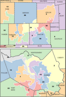
Meanwhile, Olson's, the squared-dist-based, and the splitlining maps all are pretty reasonable. Olson's map has jagged boundaries if viewed closely, which is mainly because it follows census-block-boundaries (if Olson changed his program to have it cut through census blocks, then his boundaries would smooth). Note that Olson's districts have curved boundaries (even after smoothing) while splitlining and optimizing the squared-distance-based measure both always produce district boundaries made of straight lines (on a flat Earth; on a round Earth splitlining still uses "straight" geodesic segments but the squared-dist minimizer would employ slightly non-straight curves). The basic structure of the Olson and splitline maps is almost identical, except Olson has handled the two big districts in the Western part of the state differently than (and in this case I think better than) splitlining.
And here's Virginia:
| Official | Olson |
|---|
| Splitlining |
|---|
| TX (32 districts) | Official & Olson | Splitline | Σdist²-based* | As reGerrymandered
in 2003 to favor Republicans |
|---|---|---|---|---|
| NY (29 districts) | Official & Olson | Splitline* | Σdist²-based | Census dept. provided erroneous geographic data (chopped off part of Long Island near Greenport). |
| AZ (8 districts) | Official & Olson* | Splitline | Σdist²-based | Districted by an "independent commission" (ha!); note the green district is contiguous, but joined by filaments too fine to see since <½ pixel wide. |
| IL (19 districts) | Official & Olson | Splitline | Σdist²-based* | Several too-fine-to-see filaments in the official map. |
| All 50 states | Official & Olson | Splitline | (Unrelated: what if the entire Entire USA (lower 48) were districted in 1 go? |
Here's New Jersey (also districted by an "independent commission," ha ha ha):
| Official | Olson | Splitline |
|---|
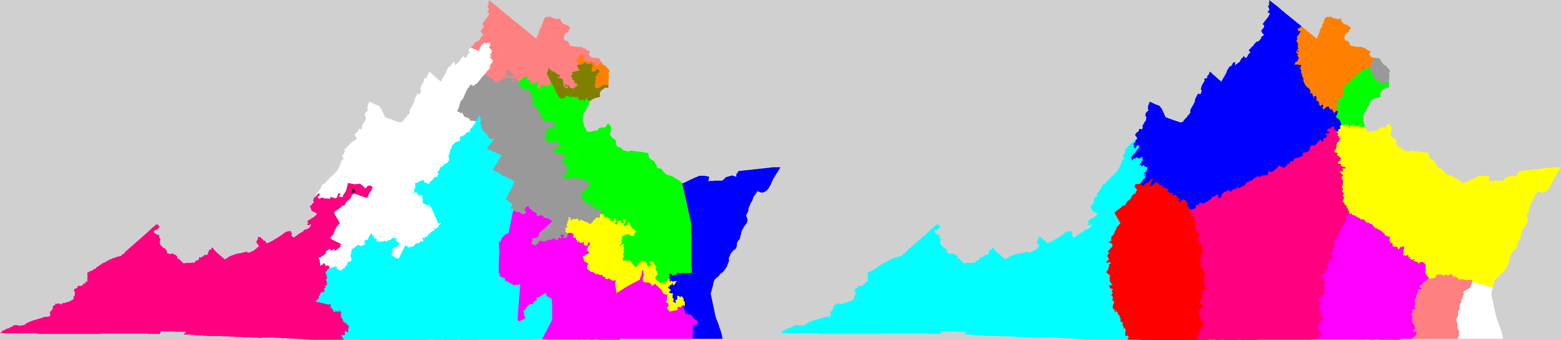
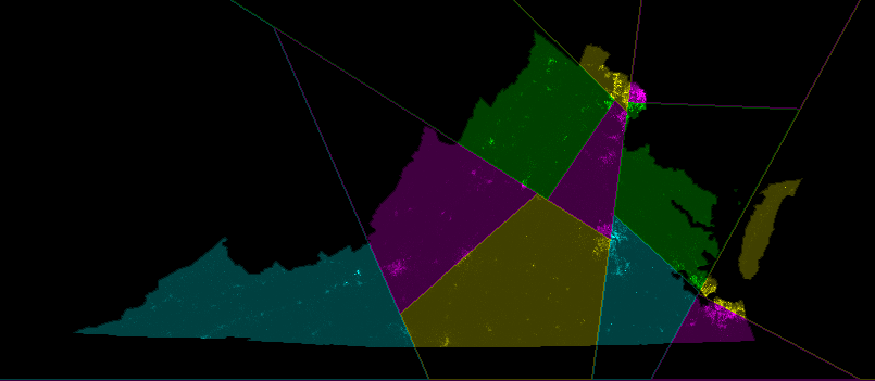
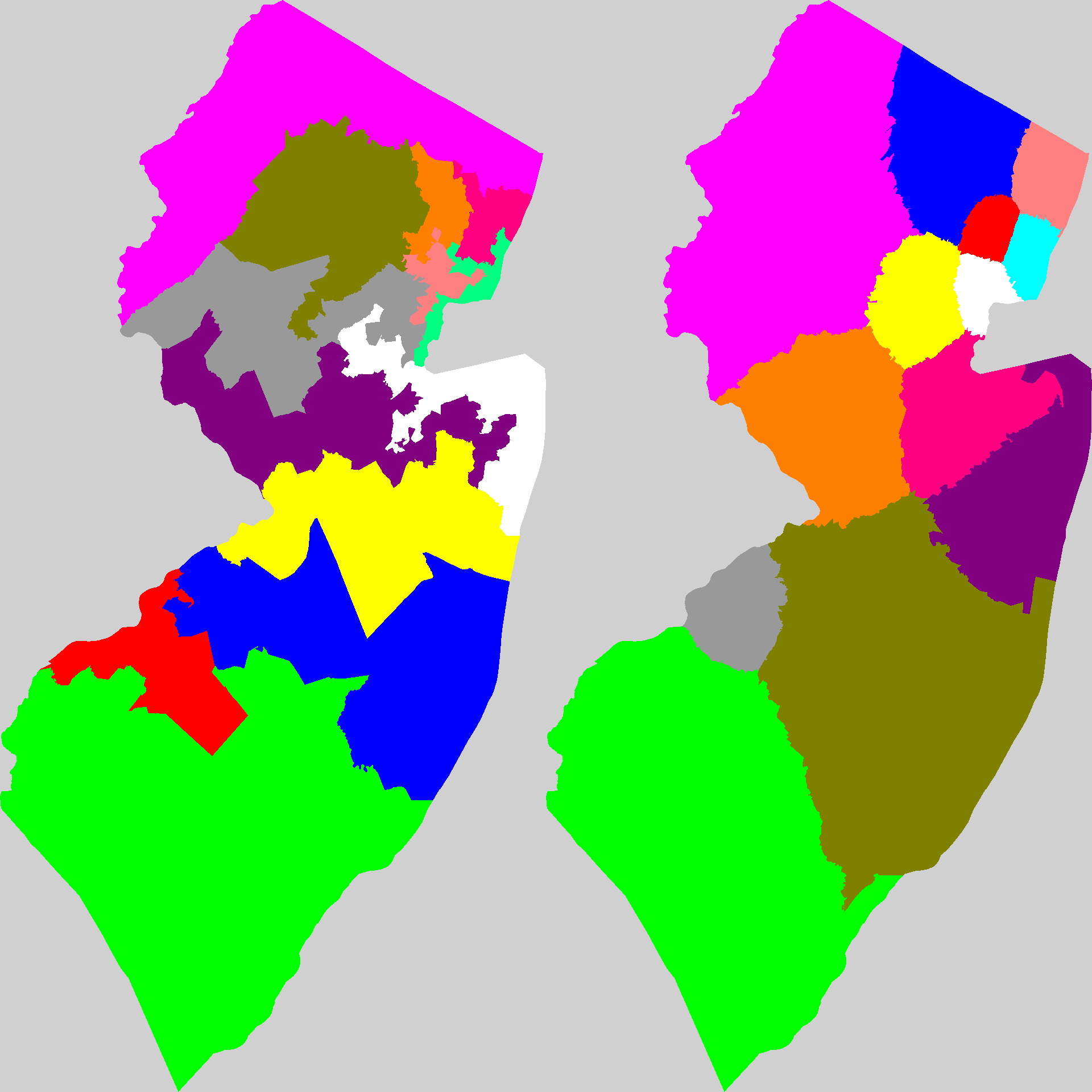
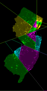
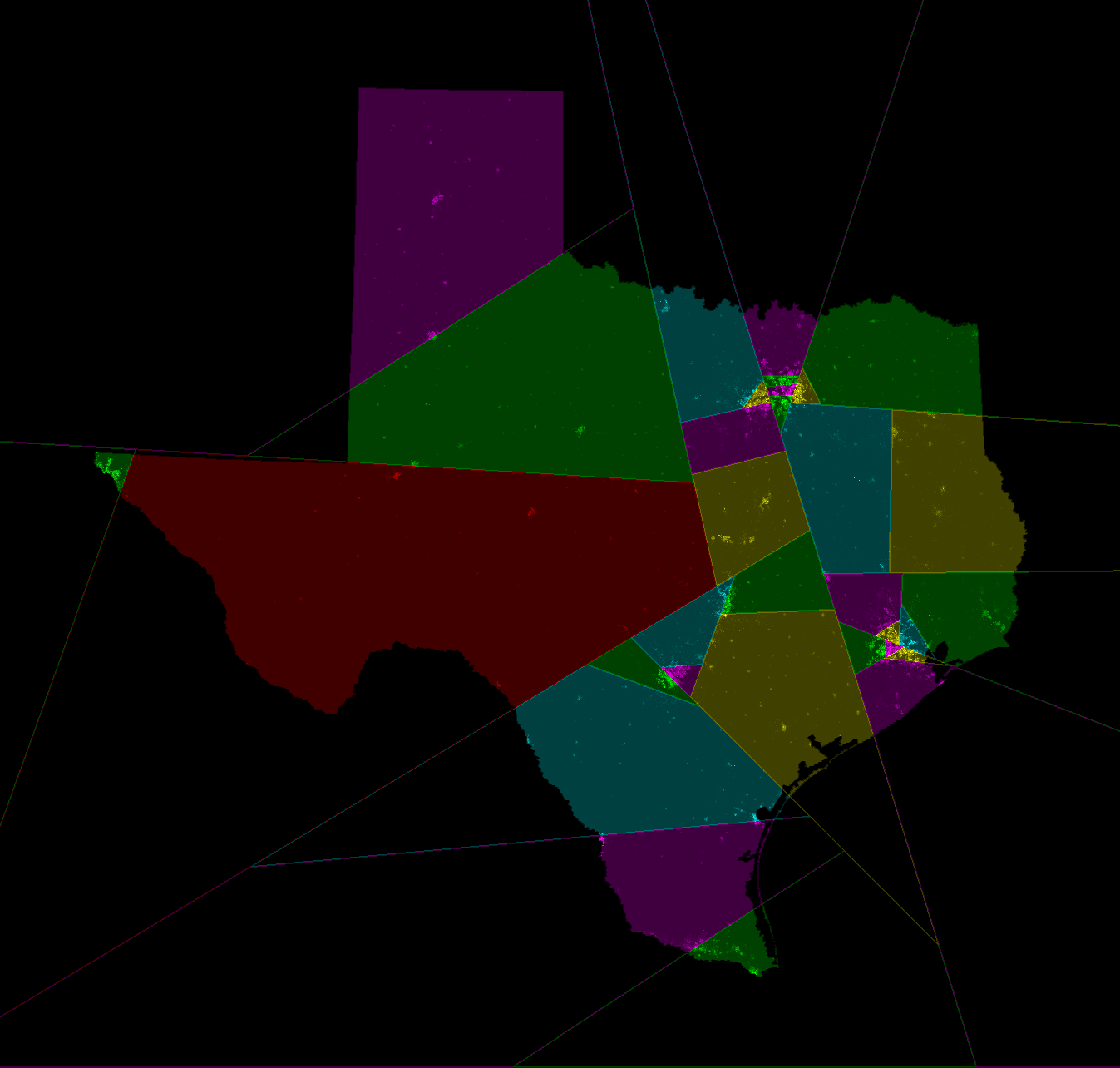
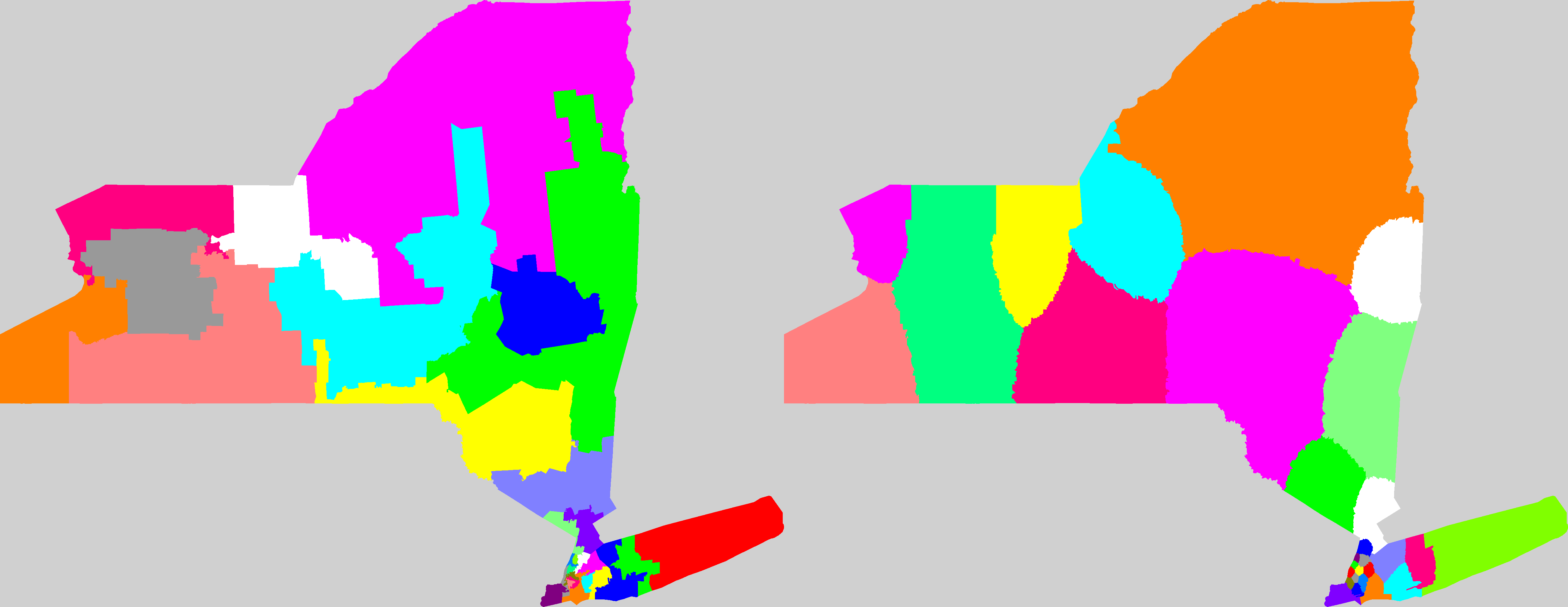
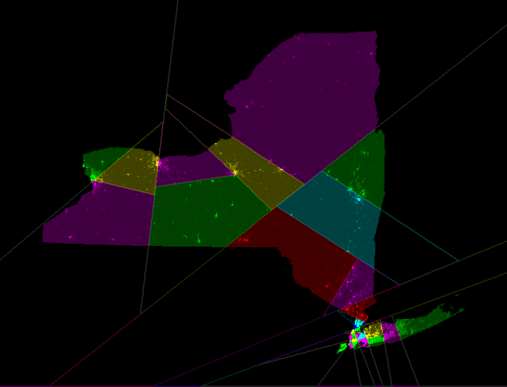
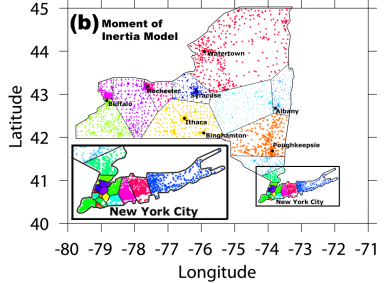
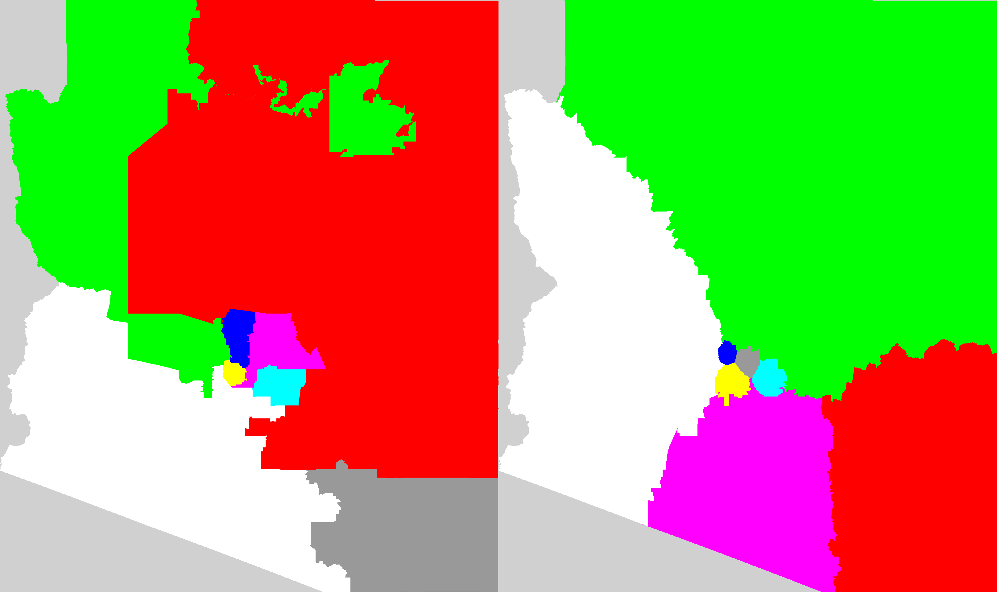
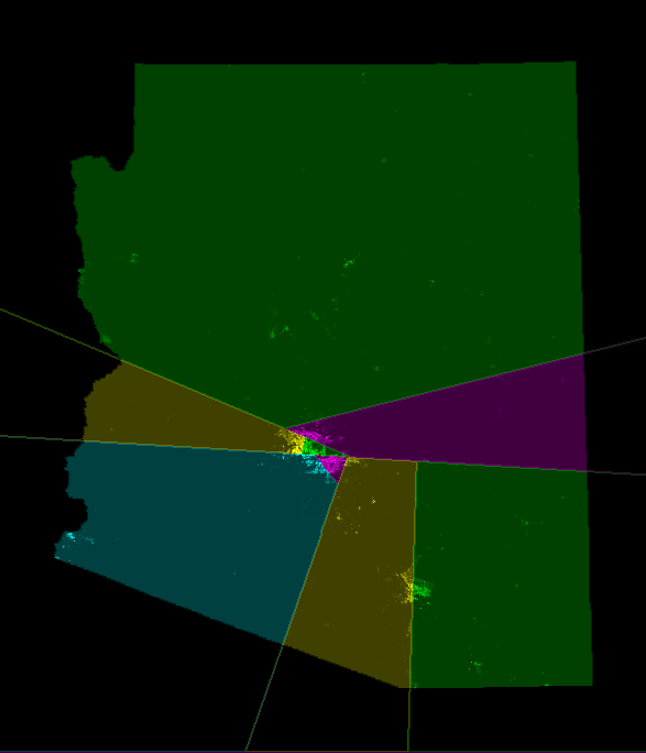
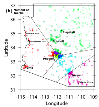
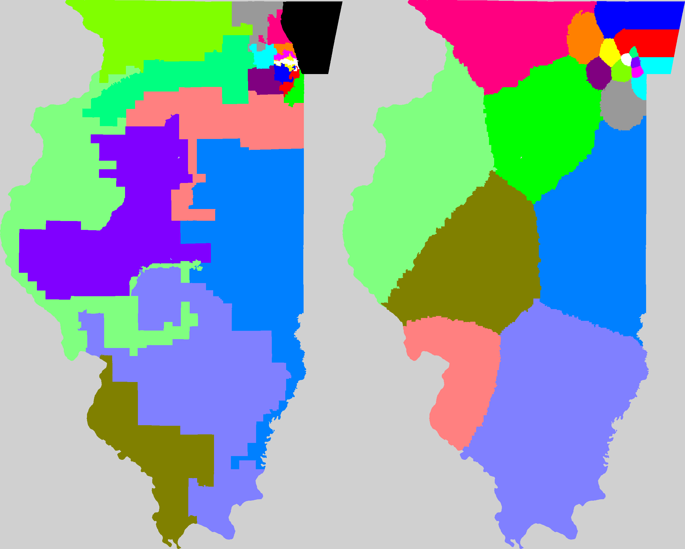
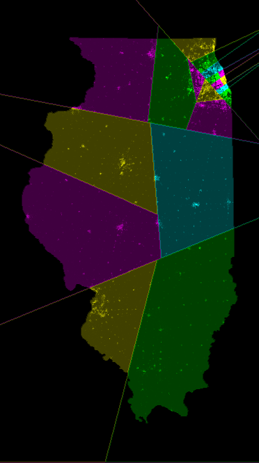
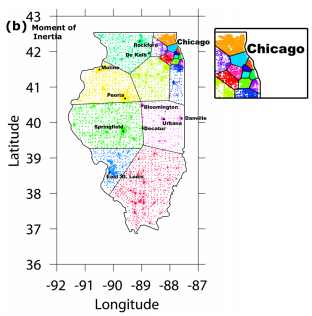
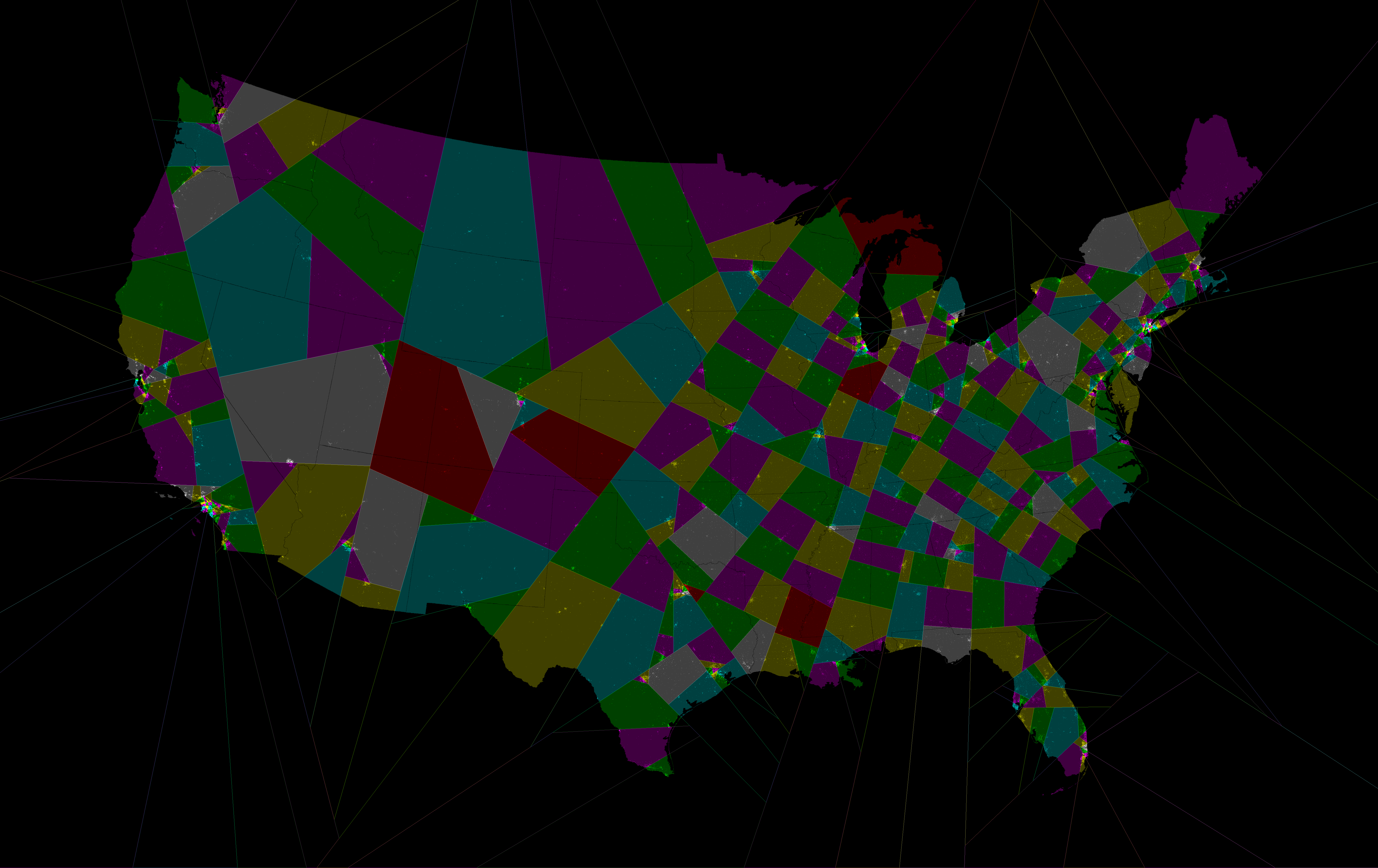