Q. I was asked to explain "Bayesian regret" and why (at least in my view) it is the "gold standard" for comparing single-winner election methods.
Oversimplified into a nutshell: The "Bayesian regret" of an election method E is the "expected avoidable human unhappiness" caused by using E.
More precise answer: Bayesian regret is gotten via this procedure:
We now redo steps 1-6 a zillion times (i.e. running a zillion simulated elections) to find the average Bayesian regret of election system E.
Comments: The Bayesian regret of an election system E may differ if we
So there are at least 5 different "knobs" we can "turn" on our machine for measuring the Bayesian Regret of an election method E.
Results of the computer simulation study: (paper #56 here). This study measured Bayesian regrets for about 30 different election methods. 720 different combinations of "knob settings" were tried. The amazing result is that, in all 720 scenarios, range voting was the best (had lowest Bayesian regret, up to statistically insignificant noise). We repeat: range was the best in every single one of those 720 with either honest voters, or with strategic voters.
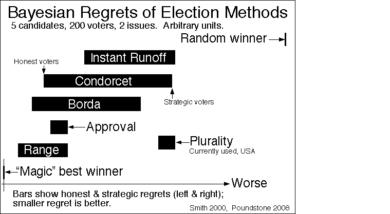
Here is a simplified table of results (from only 2 of the 720 scenarios, and only 10 of the voting systems). (Each tabulated Bayesian regret value is an average over a million or more randomized simulated elections.) Some more BR data. And some more BR data as a picture (taken from W.Poundstone's book; also available in black and white).
column A: 5 candidates, 20 voters, random utilities.
column B: 5 candidates, 50 voters, utilities based on two "issues".

                                A          B
magic optimum winner            0          0
honest range                 .04941     .05368
honest borda                 .13055     .10079
honest IRV (instant runoff)  .32314     .23786
honest plurality             .48628     .37884
random winner               1.50218    1.00462
strategic range=approval     .31554     .23101
strategic borda              .70219     .48438
strategic plurality          .91522     .61072
strategic IRV                .91522     .61072
|
Incidentally, note that with strategic voters (at least using the voting-strategy assumed by the simulation) strategic plurality and strategic IRV seem to be the same! That is because of the devastating
Theorem: Generically (i.e. if no ties), IRV and Plurality voting with strategic voters will yield the same winner in a large election: Namely the most popular among the two pre-election poll "frontrunners" will always win.
Proof sketch: For plurality voting, this was well known: strategic voters always vote for one of the two perceived frontrunners since other votes are extremely likely to be "wasted." For IRV: we again assume strategic voters will rank their favorite among the two pre-election poll "frontrunners" top, as a strategic move to maximize their vote's impact and prevent it from being wasted. [This assumption about strategic voter behavior really should have been stated in the theorem statement.] (See this example or this one to convince yourself that kind of strategy often is the unique strategically-sensible vote in the IRV system as well as many other ranked-ballot systems, and see this for data indicating the vast majority of Australian IRV voters act this way – if ≥75% act this way the theorem follows, but the data indicates 80-95% act this way.) Then the two poll-frontrunners will garner all the top-rankings from strategic voters, thus never being eliminated until the final round, whereupon the most popular one will win. (Note: actually the optimum strategy for IRV voting is not known, so my computer sim and this here theorem are assuming the "strategic voters" use this simple and not-always-optimum, IRV strategy, which however is usually a lot better than honesty, indeed see this mathematical proof it asymptotically always is optimum strategy in a random-election mathematical model subject to certain kinds of limited voter knowledge about the others.) QED.
Remark. This theorem also works for Condorcet voting (under same assumptions about voter behavior).
Bayesian "regret" (also called "loss") is just the maximum possible utility minus the Bayesian "expected utility." This is not a new concept. It dates back to the earliest days of statistics (1800s) and it has been used in at least a dozen papers on non-voting-related subjects. The only thing "new" here is applying this well known concept to voting methods. And that idea also was thought of by others besides me, e.g. Merrill and Bordley.
Let's make a quick estimate to translate this into pocketbook terms.
Suppose thanks to a poor voting method, our elections 5% of the time make avoidable bad decisions. That has an effect analogous to a 5% tax on society. Unlike a real tax, though, this tax does not get used for any useful purpose, it just gets wasted. And furthermore this is a stupid waste – that could have been trivially avoided by adopting better voting systems. Over time, that 5% keeps adding up and up. After a century of annual compounding, 5% interest would represent a multiplicative factor of 132. That is, your country, by the trivially easy move of adopting (versus not adopting) a better voting method, would under this estimate be one hundred and thirty two times richer. If however this 5% bad-decision rate were only equivalent to a 1% tax, then we'd only get 2.7 times richer. Either way, this is a massive improvement for very little effort.